- Mon 27 October 2025
- machine-learning
- #ai, #data, #machine-learning, #pytorch, #xournalpp-htr, #visual, #didactical, #computer-vision, #segmentation, #clustering
Try 🤗 HuggingFace demo & 👩💻 Code on Github & 💬 Send me feedback
Ever wished your handwritten Xournal++ notes were searchable like typed documents? That’s exactly what my tiny open-source Xournal++ HTR project aims to solve using modern machine learning.
As part of professionalising Xournal++ HTR, I re-implemented Harald Scheidl’s fantastic WordDetectorNet model for detecting handwritten text on pages using PyTorch. Finding where words are located on a page is the first crucial step in making handwritten notes searchable.
I really liked the idea behind WordDetectorNet. I want to share a visual explanation of how WordDetectorNet works in this blog article because I learned quite a bit while re-implementing it.
Useful details outside the direct explanation of WordDetectorNet are covered in expandable excursion boxes denoted by the ⭐️ emoji.
Problem Setting
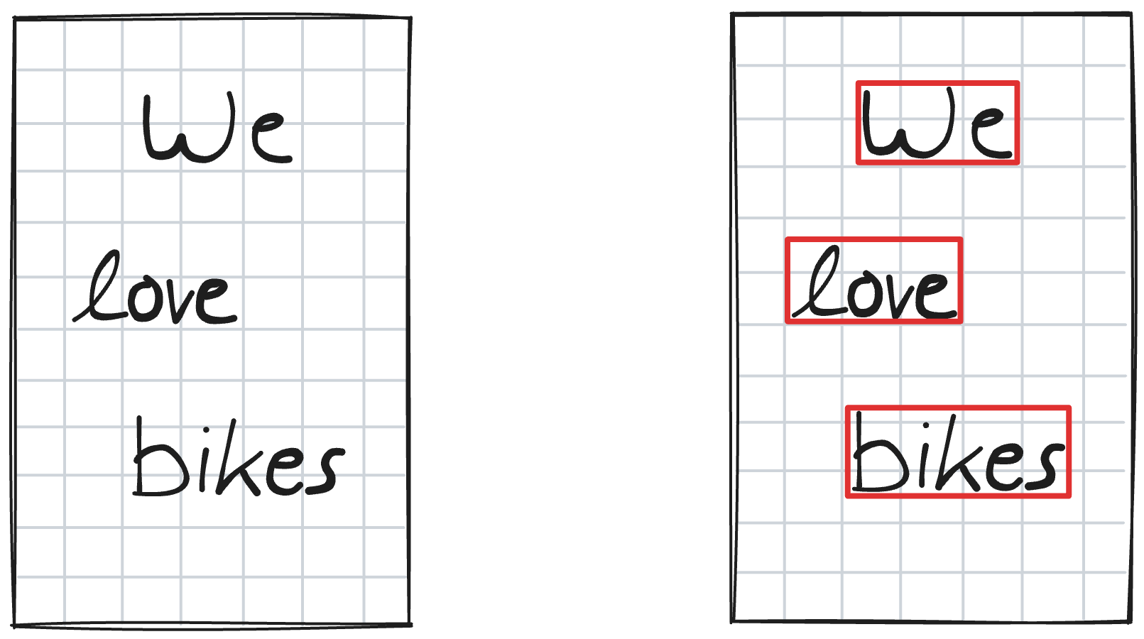
Given an image with handwritten text on, we want to use the WordDetectorNet to predict the bounding boxes around all words as a list.
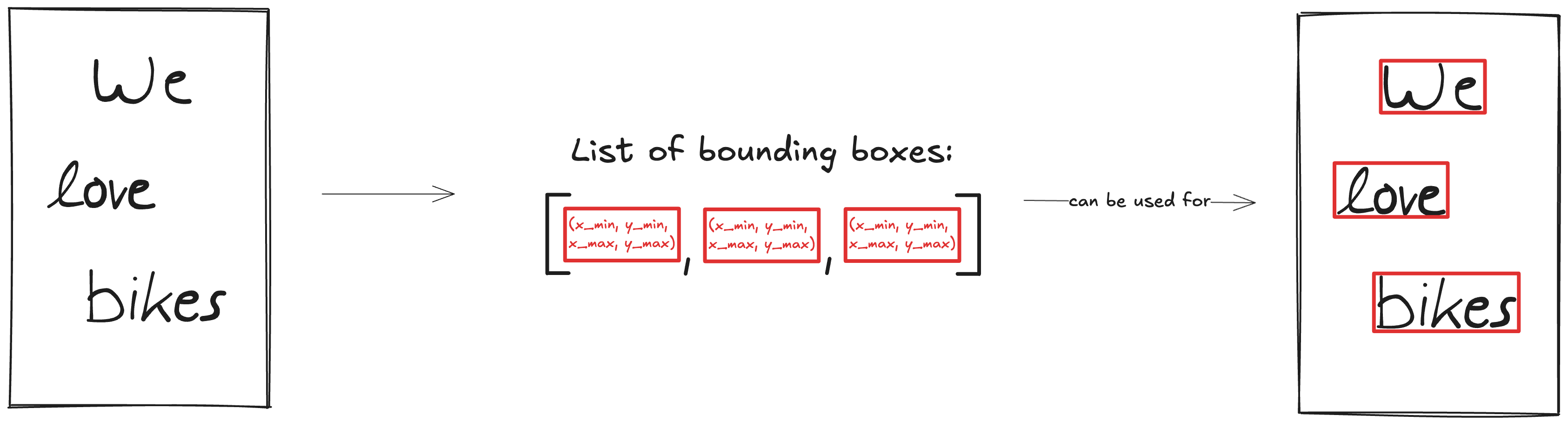
This list of bounding boxes can then conviently be used to draw the bounding boxes around words.
The WordDetectorNet is the first part of the machine learning pipeline in the Xournal++ HTR project to make handwritten notes searchable. WordDetectorNet finds all words on a page and forwards them to a subsequent model which transcribes the actual text from images of words to strings. Although I don’t cover the transcription part in this blog article, you can try a full end-to-end open-source demo of the Xournal++ HTR project for text recognition using this 🤗 HuggingFace demo.
⭐️ Excursion: What is a bounding box?
A bounding box represents a rectangular region on an image that contains an object of interest. We follow the standard computer vision convention where the coordinate system has its origin (0, 0) at the top-left corner.
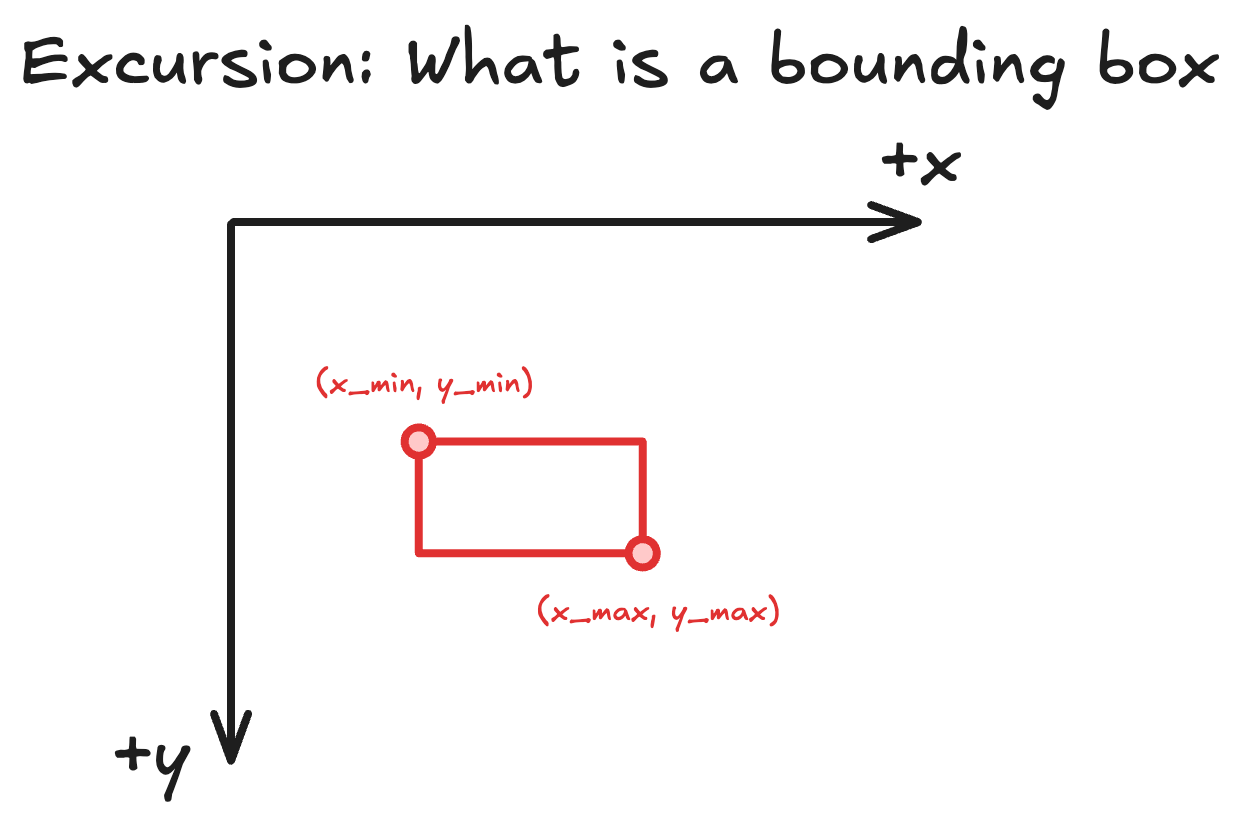
Every bounding box is defined by exactly 4 values. These can be represented in different ways: either as a top-left point plus width and height, or as minimum and maximum coordinates for each dimension. Throughout this article, I use the latter format: (xmin, xmax, ymin, ymax).
Solution Overview
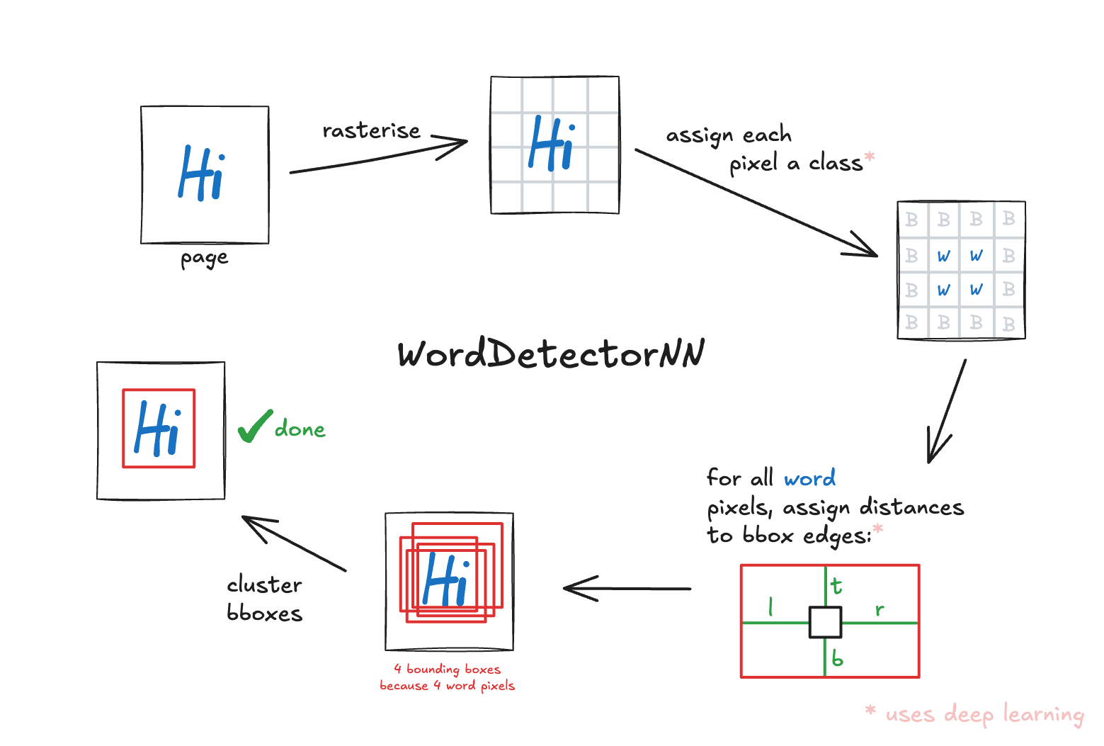
WordDetectorNet solves finding words on pages using a two-stage pipeline: a deep learning model followed by a clustering step. The deep learning component does most of the heavy lifting, while the clustering helps refine the final results, see the overview figure below.
This article is structured in two main parts. First, I’ll walk you through the complete pipeline, explaining how the deep learning and clustering steps work together - this is where most of the interesting modeling happens. Then, we’ll take a deeper look into the neural network architecture itself, which uses a ResNet18-based encoder combined with a Feature Pyramid Network decoder to generate pixel-wise predictions.
Step-by-step Explanation
Before looking at the complete pipeline that uses deep learning and clustering, it’s worth to mention some background to bring everyone on the same page.
Background
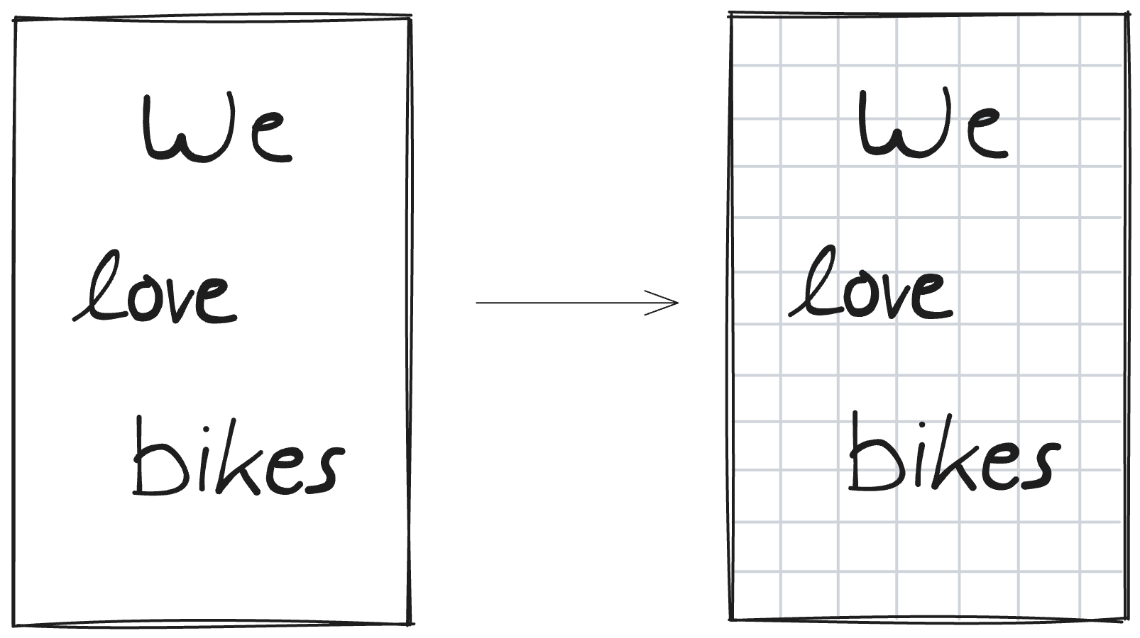
An image, like a scan of handwritten text, consists of pixels; denoted by gray boxes in the following image.
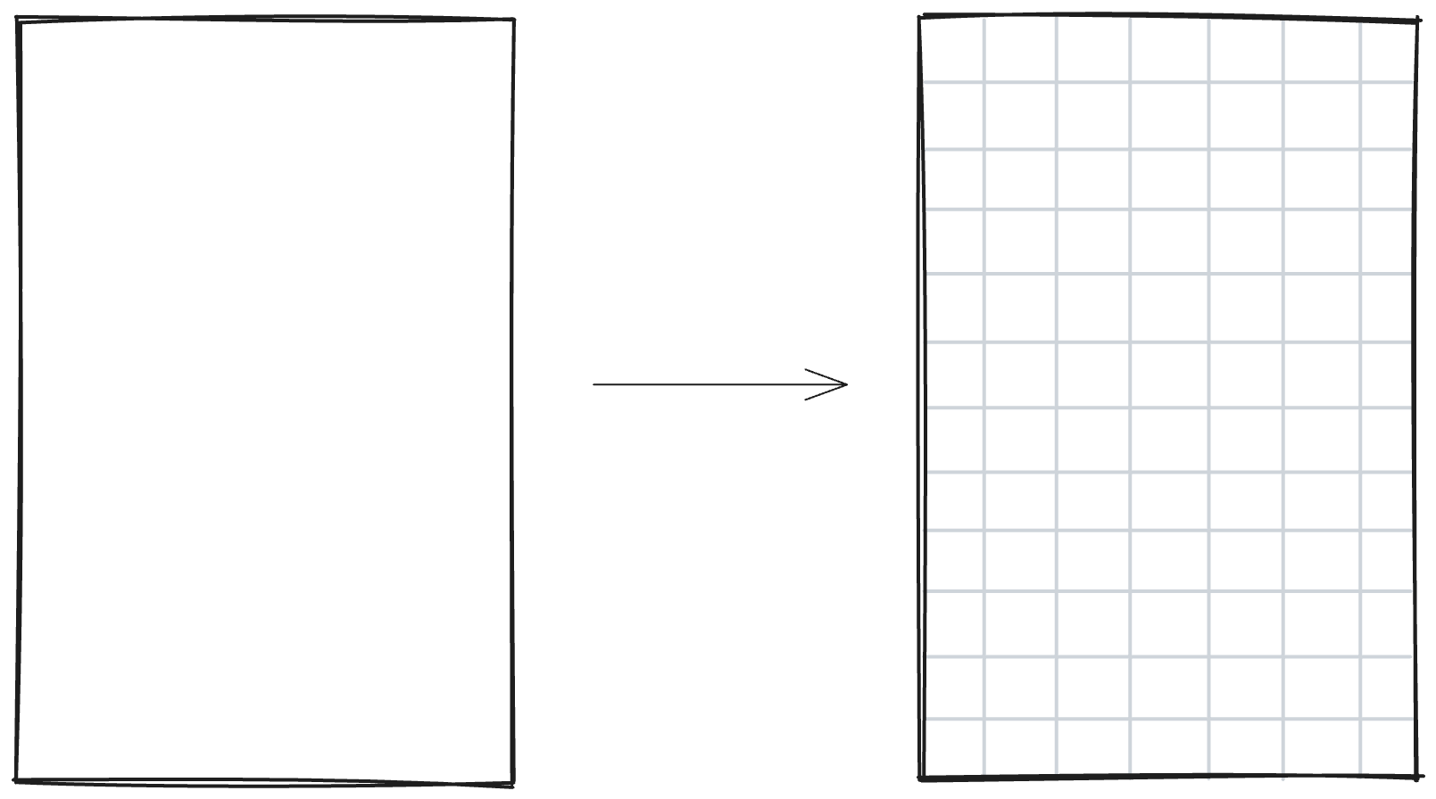
Handwritten text on a page therefore lives in this pixel space. The example shows handwritten text “We love bikes”. Of course, normally there are many more pixels so that they actually make up the strokes and can resolve them.
After training, the WordDetectorNet will find the bounding boxes around the words and, as is the case in the Xournal++ HTR setup, return them as a list for transcription.
WordDetectorNet Modeling Approach
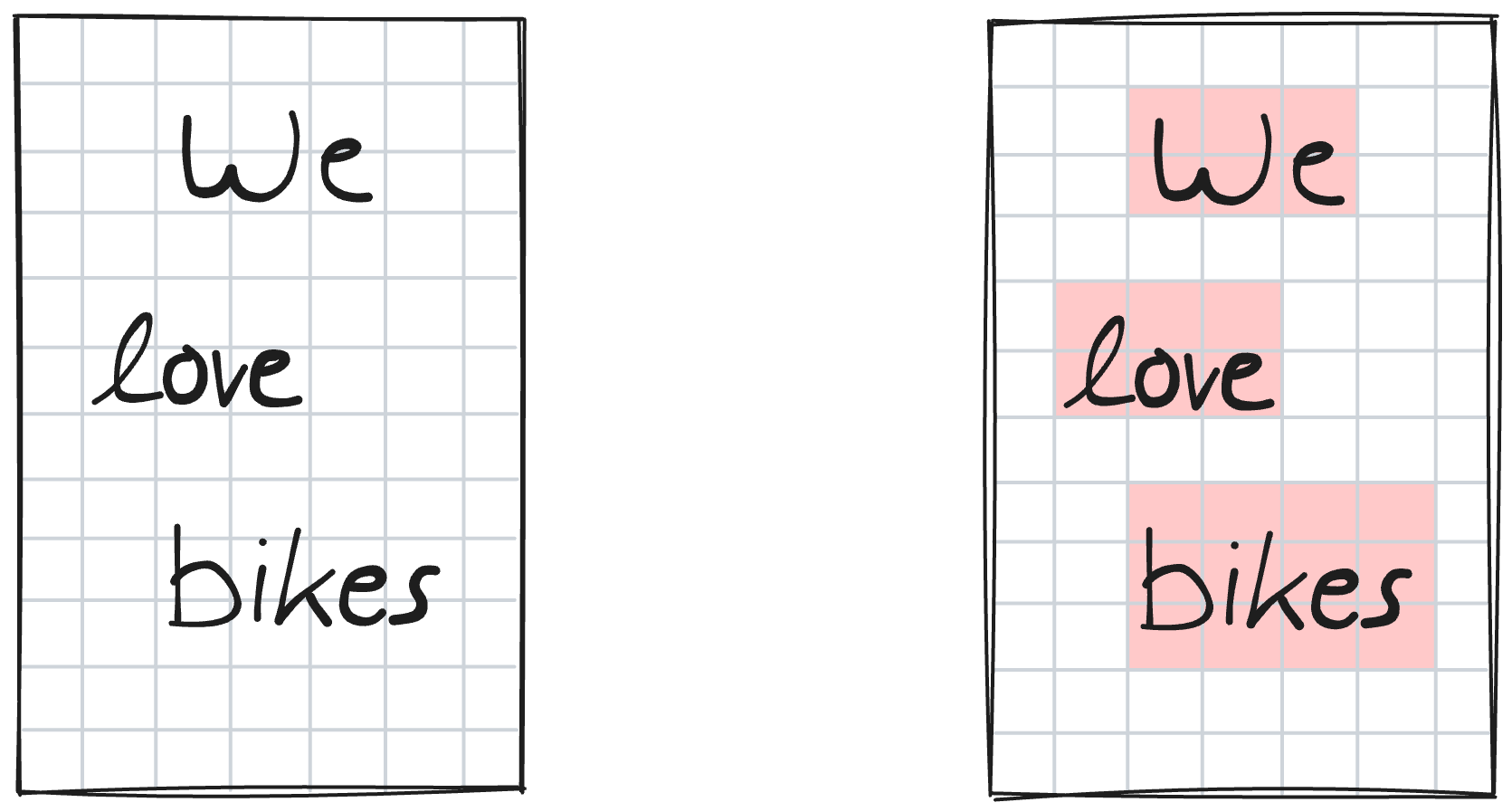
Each pixel on the page is assigned a class. This is called a “segmentation task”. In the following figure, red denotes “word pixel” and white “background pixel”.
⭐️ Excursion: Classification with deep learning
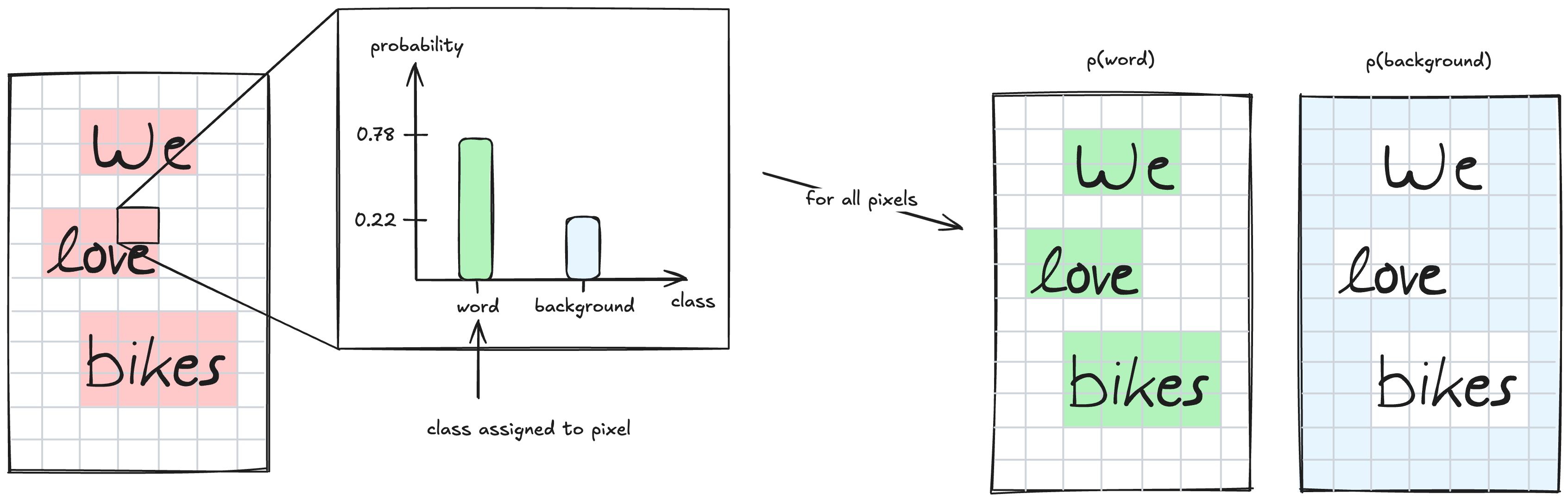
Classification in deep learning is typically done by predicting a probability distribution. Here, there are two possible outcomes for each pixel: “is background” and “is word”. Therefore, the model predicts two probability values for each pixel that sum to 1. When the prediction is performed for all pixels across the image, it creates two output maps that contain these probabilities.
Now we have bounding boxes as a segmentation mask. But we actually want a list of bounding boxes, not a pixel-wise segmentation. We’ll need a post-processing step.
To solve this, we assign each pixel not only a class, but also its relative position within the bounding box if it is a “word” pixel. The following figure shows how a “word” pixel is assigned relative distances of 1 to the top of the bounding box, 2 to the right, 1 to the bottom, and 1 to the left.
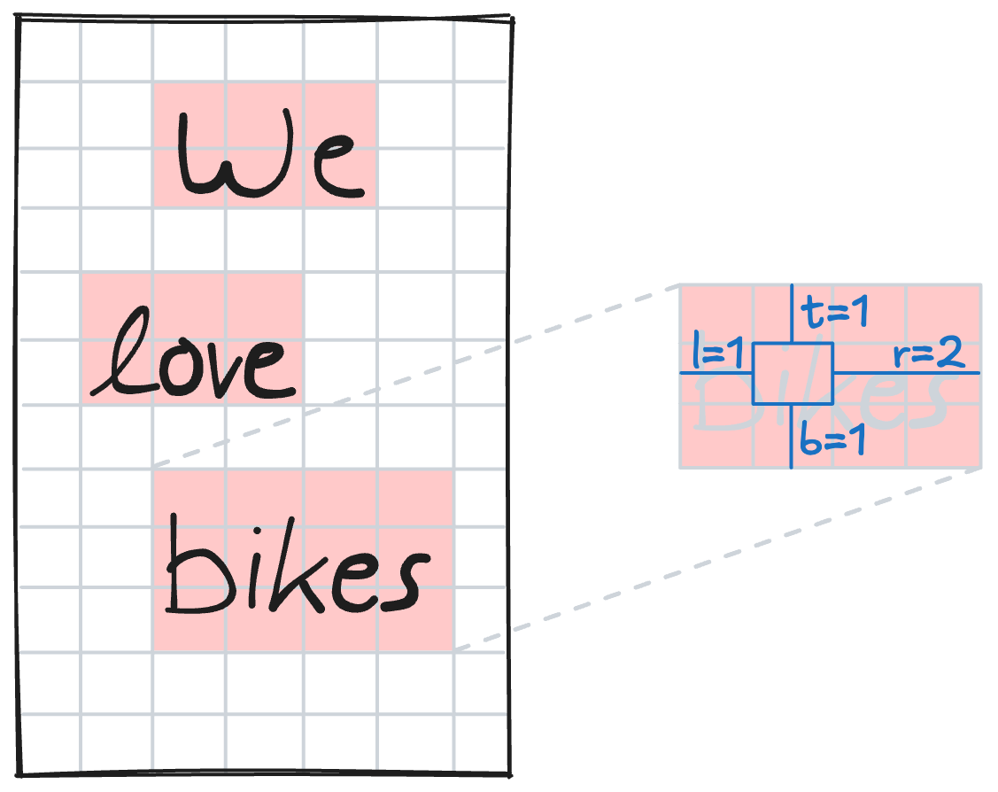
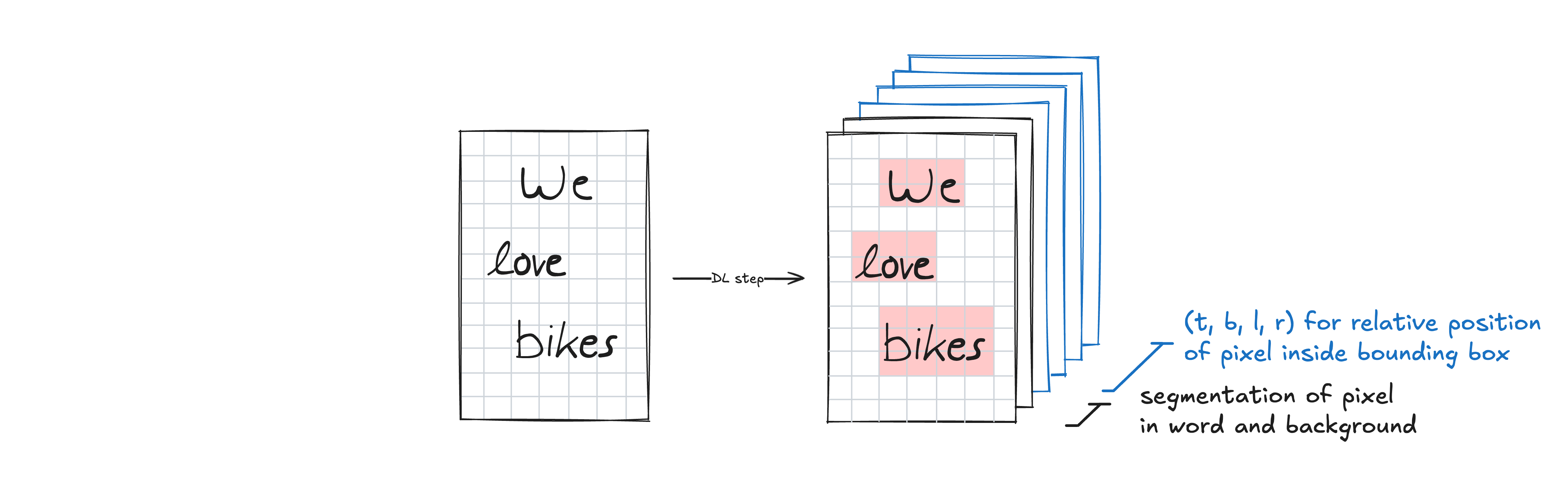
This is the core output of the deep learning step: every pixel is assigned 6 values by the neural network. Specifically, 2 values for one-hot encoded segmentation (i.e. the pixel-wise classification explained above) and 4 values for relative position within the bounding box through distance measurements. This transforms one input image into 6 predicted output maps.
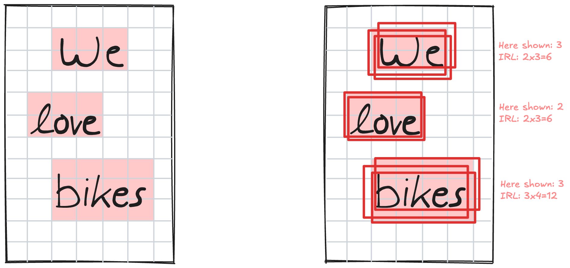
From each word pixel, we can use its distance values (top, bottom, left, right) to reconstruct a complete bounding box. This means we generate as many bounding boxes as there are word pixels. In our example there are 12 word pixels for the word “bikes” and therefore we get 12 predicted bounding boxes for this word. Ideally, all these bounding boxes would be identical, but in practice they vary slightly while having significant overlap.
Using the output of the deep learning model, we have now reconstructed a list of many parametric bounding boxes - one for each word pixel on the page. The bounding boxes that correspond to the same word overlap significantly while bounding boxes for different words have no overlap.
All that is great but there’s still one issue: we have multiple bounding boxes for each word when we only want one per word!
This is where clustering comes to the rescue. Since we don’t know how many final bounding boxes we should have (i.e., how many words are on the page), we use DBSCAN as our clustering algorithm.
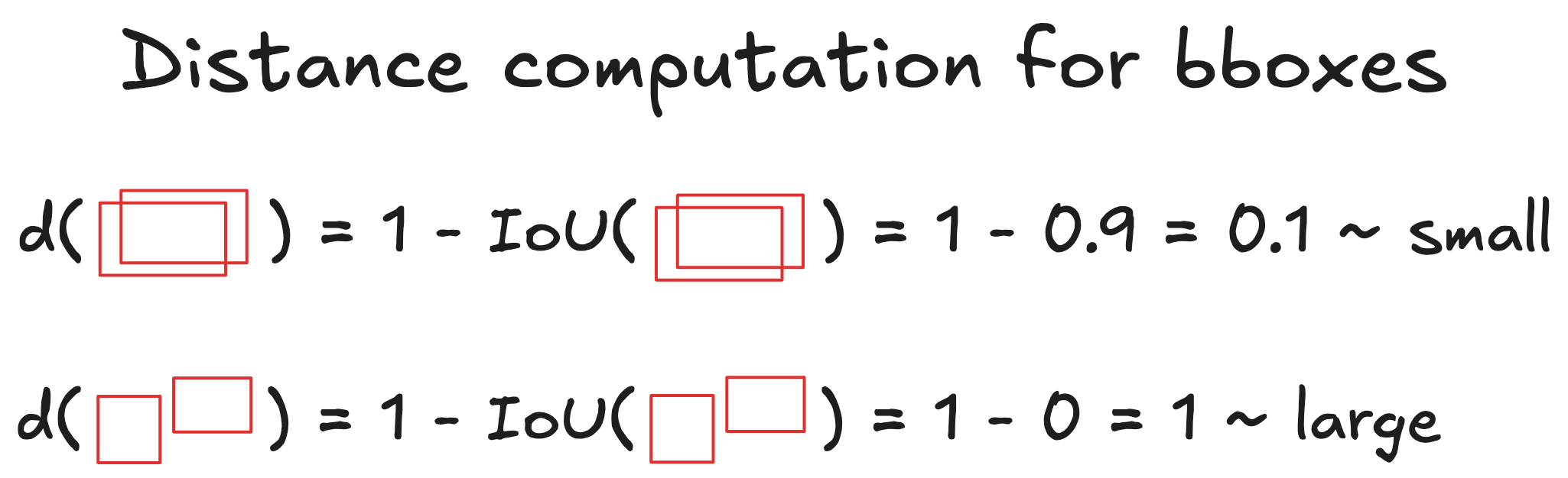
DBSCAN requires a “distance metric” to measure how similar objects are for clustering purposes. We define the distance between two bounding boxes based on their overlap: specifically, the distance equals 1 minus their Intersection over Union (IoU). With this metric, overlapping boxes get assigned small distances (close to zero) while separated boxes get large distances (close to one).
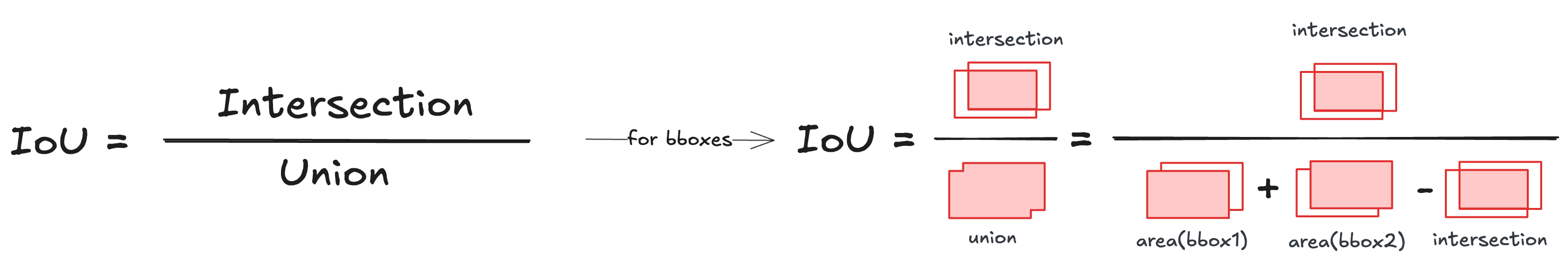
⭐️ Excursion: Intersection over Union (IoU)
Intersection over Union (IoU) is a common metric used in object detection and image segmentation that measures the overlap between two shapes like bounding boxes. It’s calculated as the area of intersection divided by the area of union between two shapes.
We compute the distance between all pairs of bounding boxes and store the results in a distance matrix, which serves as input to the DBSCAN algorithm. In the distance matrix visualization below, brighter colors represent bounding box pairs that are closer to each other because of overlap.
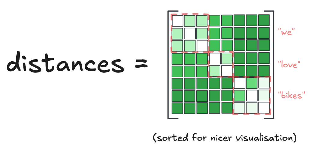
We can clearly recognise the three distinct clusters in our example that correspond to the three words on the page (see the dashed red boxes and corresponding words next to matrix for extra clarity), with the diagonal values being 0 because the distance of a bounding box to itself is 0. Interestingly, the pairwise distance calculation is currently the computational bottleneck of the model because it scales quadratically with the number of predicted bounding boxes (which can be quite large).
DBSCAN then assigns each bounding box to a cluster. For each cluster, we compute the final bounding box by taking the median of all bounding box coordinates within that cluster.
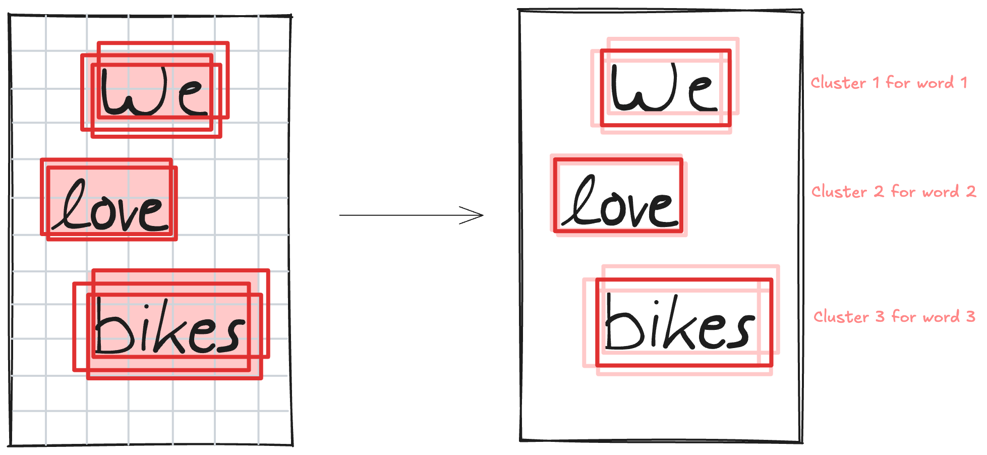
That’s it! We have successfully obtained a list of parametric bounding boxes on a page, one for each word.
What’s particularly interesting is that most of the modeling approach isn’t purely deep learning - it’s actually a clever combination of a neural network with a traditional clustering algorithm. Now let’s explore how the neural network component generates those pixel-wise segmentation masks and bounding box parameters.
Neural Network Architecture
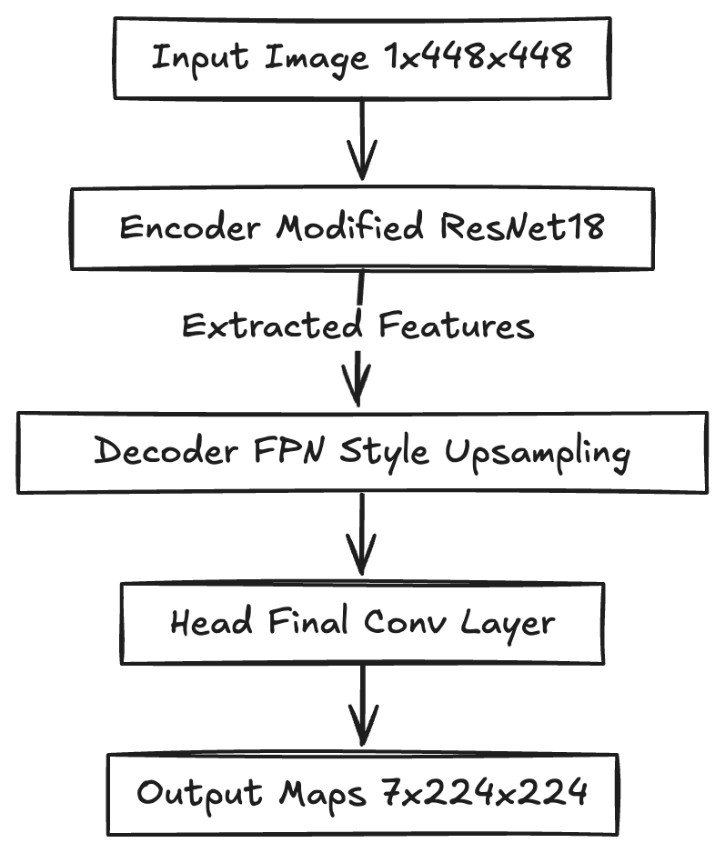
The deep learning step takes an input image and produces 6 output maps at lower resolution, each containing different types of information about the words on the page.
You’ve seen this visualization before - it’s the high-level overview of what the neural network accomplishes:
⭐️ Excursion: The ResNet18 architecture
The ResNet18 is part of the ResNet family of networks introduced by He et al in 2015 [ResNets]. They are convolutional neural networks that introduce skip connections to overcome performance degradation in deep networks.
The following image shows the high-level architecture of ResNet18, which consists of 5 convolutional blocks and a classification head at the end.

The deep learning part model uses the ResNet18 model as its backbone. In computer vision, a backbone is the foundational feature-extraction part of a deep learning model, typically a pre-trained network, that converts a raw input image into high-level feature maps for specific tasks like detection or classification.
The WordDetectorNet uses this ResNet18 backbone to extract features and then applies the Feature Pyramid Networks [FPN] concept to create high-dimensional, semantically rich maps that are used to compute the 6 output maps.
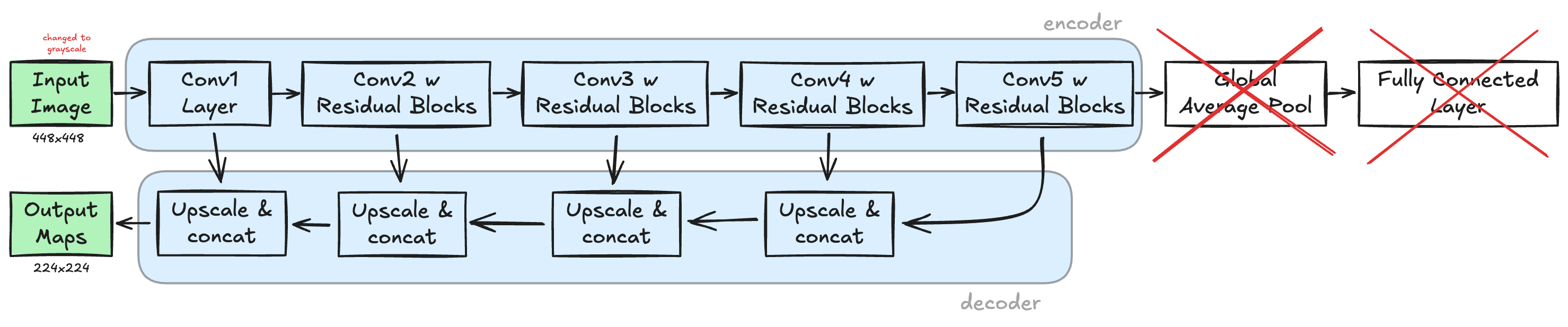
The WordDetectorNet architecture removes the original classification head of the ResNet18 architecture and instead up-scales and concatenates the features from all convolutional blocks of the ResNet18 to obtain scale-invariant features that ultimately produce the 6 output maps. Therefore, the ResNet18 part of the WordDetectorNet acts as encoder and is followed by a decoder to obtain the 6 output maps.
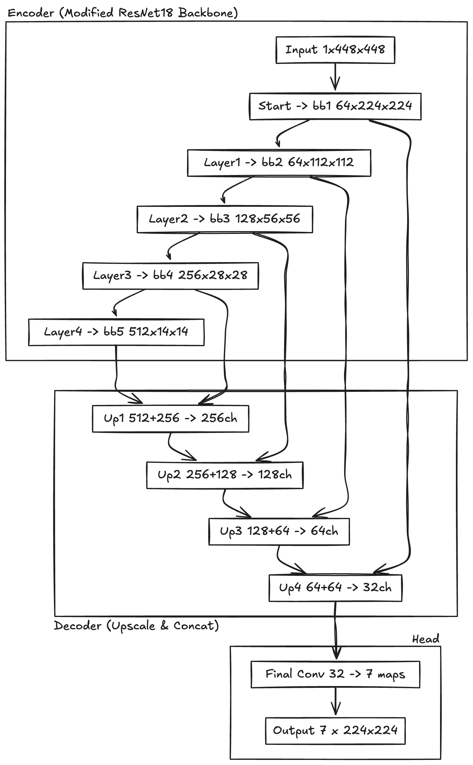
⭐️ Excursion: Full architecture with convolutional shapes
I provide two depths of architecture explanations, one with less and the other with more details.
The WordDetectorNet architecture comprises of an encoder-decoder architecture based on the Feature Pyramid Networks [FPN] idea with a modified ResNet18 as feature encoder and simple upscaling and concatenations as decoder. A final head then maps the features into the desired shape of 6 output maps.
Now in more detail: The backbone is a modified ResNet18 with two changes. First, the number of input channels is changed from 3 to 1 in order to accept grayscale images natively rather than RGB images. Second, the forward implementation has been changed to return the features after each residual block to obtain features at different scales. These features are then used in the decoder part of the architecture.
To complete the explanation of the neural network, I still need to discuss two key aspects: the loss function and the dataset used.
The loss function has two equally weighted parts, namely a segmentation loss (using cross-entropy) and a geometric loss (using the Intersection over Union measure presented earlier). The segmentation loss makes sure that pixels are classified correctly and the geometric loss makes sure that the WordDetectorNet can predict relative positions of word pixels inside bounding boxes.
The whole system was trained using the IAM Handwriting Database [IAM]. This dataset is reformatted into a list of tuples with grayscale images as input to the network and a list of bounding boxes as target output. The input images are resized to a size of 448x448 pixels and the target output is converted into a 6-channel image of size 224x224. Harald’s implementation added image augmentations to improve performance but I have not done so yet.
Conclusions
WordDetectorNet demonstrates an elegant hybrid approach to find handwritten words on a page by combining deep learning with traditional clustering.
The main limitation of its approach is, however, the clustering step because it introduces additional hyperparameters that prevent end-to-end learning and because of the quadratic complexity to compute pairwise distances between all bounding boxes. A good alternative might be YOLOv8s, which has more weights and FLOPs than WordDetectorNet but can be trained end-to-end & doesn’t require a costly clustering step at the end of a pipeline forward pass.
Thanks to Harald Scheidl for this excellent architecture and making it open source!
This explanation of WordDetectorNet is just one part of the broader open-source Xournal++ HTR project.
If you’d like to support the work, consider starring the repository on GitHub to help increase its visibility, contributing code or ideas, or exploring the Xournal++ HTR demo on Hugging Face. You can even choose to donate handwriting samples to help improve the underlying machine learning models for everyone.
A brief clarification: there are actually three segmentation classes, not two. The third class corresponds to boundary pixels, resulting in seven output maps. I omitted this in the present blog article to keep the explanation focused.
References
- [ResNets] He, Kaiming, Xiangyu Zhang, Shaoqing Ren, and Jian Sun. “Deep Residual Learning for Image Recognition.” 2016 IEEE Conference on Computer Vision and Pattern Recognition (CVPR), IEEE, June 2016, 770–78. https://doi.org/10.1109/CVPR.2016.90.
- [FPN] Lin, Tsung-Yi, Piotr Dollár, Ross Girshick, Kaiming He, Bharath Hariharan, and Serge Belongie. “Feature Pyramid Networks for Object Detection.” arXiv:1612.03144. Preprint, arXiv, April 19, 2017. https://doi.org/10.48550/arXiv.1612.03144.
- [IAM] IAM Handwriting Database
Thanks to Linda Nguyen for early review of this blog article.
Please hit me up on LinkedIn or email for any corrections or feedback.